Which is the most distant 2-digit number from any 1-digits?

One of my recent hobby is to think of fun math problems to encourage our 6-year-old daughter to play with the virtue of numbers. At the moment she knows of multiplication and division between pairs of 1-digit integers as the most advanced topic to her.

When I talked with her over 9×9 multiplication table—a standard material for elementary math in my country—, I realized that any 2-digit integers converge to an 1-digit integer after repeatedly applying a certain operation. The operation is quite simple; take the first and second digits and multiplying them. For example, the operation, let us call it the digit multiplication hereafter, transform 23 into 2×3 = 6, 54 to 5×4 = 20, and so on.

Let us quickly recap that any 2-digit integers eventually converge to 1-digit with this. A 2-digit integer is represented as 10a+b with a, b = 1, 2, …, 9. Then, the digit multiplication converts 10a+b to ab. It is straightforward to see following two properties of the digit multiplication. First, the resultant ab is bounded from both sides as 1 ≤ ab ≤ 81. Second, the digit multiplication always returns output smaller than its input: the difference is negative as ab – (10a+b) = (a-1)b – 10a ≤ 10(a-1) – 10a = -10 (the equality holds iff a = 1). These two properties ensure that the digit multiplication transforms any 2-digit integer into 1-digit after some iterations, at most 8 times (a rough estimation).

Now if we take the number of iterations required to reduce a 2-digit integer into an 1-digit as its "distance" to any 1-digits, we can find the most distant 2-digit among 10 to 99. To find the extreme one, should we apply the digit multiplication for several times until all the results become less than 10? Definitely not! Instead, we apply the digit multiplication only once and then draw a network between numbers.

The whole space of operating the digit multiplication is represented as 10 directed trees between numbers in which a directed edge is drawn from input to output such as 23 → 6 and 54 → 20 and the roots of which are 0 to 9, i.e., the destinations. Following visualizations tell us how these trees look like:
component0component1component2
component3component4component5
component6component7component8
component9

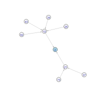
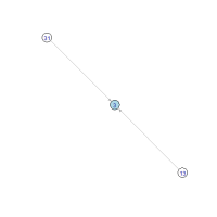
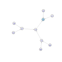
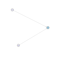
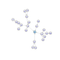
Apparently the trees of root 0, 6, and 8 are the largest ones. By contrast, the trees of root 1, 3, 7, and 9 are the smallest ones, surrounded by only a few primes (except 33 and 91). We seem to come to the roots in a few steps wherever we start at and the most distant one may be in the trees of 0, 6, or 8.

The answer to the most-distant-one question becomes crystal clear when we plot the 2-digit integers and its distance to the nearest root as follows:

The answer is 77! Among 10 to 99, only 77 requires 4 steps to come to 8, via 77 → 49 → 36 → 18 → 8. Now dad keeps this new piece into his “fun-math-fact” list to show it to daughters someday…

Below is the script to reproduce the figures:

library(dplyr)
library(ggplot2)
library(ggthemes)
library(igraph)
library(glue)

# Set the data
x <- 0:99
y <- ifelse (x < 10, NA, (x %/% 10) * (x %% 10))
df <- data.frame("x" = x, "y" = y)

# Create a directed graph from the data
g <- graph.data.frame(df %>% filter(!is.na(y)), directed = TRUE)

# Find 10 components (directed & rooted trees) in g
c <- components(g)

# Plot each tree
for (cid in 1:10) {
  cc <- induced.subgraph(g, vids = V(g)[c$membership == cid], impl = "copy_and_delete")
    
  png(glue("./R/plot_component{cid-1}.png"))
  plot.igraph(x = cc,
              vertex.color = ifelse(degree(cc, mode = "out") == 0, "light blue", "white"),
              vertex.label.family = "sans",
              edge.arrow.size = 0.5)
  dev.off()
}

# Plot the distance from leaves to the nearest root (1-digit number)
d <- distances(graph = g, v = V(g)[1:90], to = V(g)[91:100], mode = "out")
dmin <- apply(X= as.matrix(d, ncol = 9), MARGIN = 1, FUN = min)

ggplot (data = data.frame(x = as.integer(names(dmin)), y = dmin),
        aes(x = x, y = y, color =y)) +
  geom_segment(aes(x = x, y = 0, xend = x, yend=y), size = 1.2) +
  geom_point(size=3, color = "grey40") +
  xlab("2-digit number") +
  ylab("distance to the nearest 1-digit number") +
  scale_color_continuous(low = "grey", high = "#0072B2") +
  guides(color = FALSE) +
  theme_minimal(base_size = 15)

Advantages to be an interdisciplinary being (on a transition to the industry)

8月の後半、国際学会に参加するためにロンドンに行った。到着したその足で会議場そばのホテルへ向かい、スーツケースを部屋において水と食料を調達しに外へ出かけた。ホテルのロビーからエントランスへ降りるエレベーターで、2人連れの女性と乗り合わせた。「私たちは教育関係のカンファレンスで今日まで来ているんです。あなたも何かの会議ですか?」自分の母親と同年代と思われる方に尋ねられ、(この疲れているときにエレベーターピッチとは…人生は厳しい)と思いながらも返答に詰まった。この初対面で何も共通の関心が見当たらない人に、自分の専門をどう表現したらいいものか。その…と数秒時間を稼いで口をついた答えは「コンピュータサイエンスです」だった。これには自分自身でがっかりした。本当の専門分野は、いわゆるコンピュータサイエンスとは相当の隔たりがある。とっさの事だし仕方がないと思いながらも、代わりに何と答えれば十分な返答だったのだろうと考えていた。

そんな記憶がまだ新しいうちに、佐山弘樹さんが Twitter に投稿されていた講演資料に目が止まり、スライドを一息に読んだ。学際的(interdisciplinary)研究者として生き残るためのヒントが、ご自身の実体験に基づいて書かれてある。(個人的には、佐山さんとは2012年頃から国際学会でお会いすると食事をご一緒したり良くしていただいていて、その意味でもスライドから活き活きとしたトークの雰囲気を感じながら読んだ。)

スライド中、”Challenges” の節にまず取り上げられる identity crisis は、ああ正に先日の自分のことだと実感をもって同意する。今回だけでなく「何の研究をしているんですか」と聞かれて相手が得心するような答えを返せなかった経験は少なからずある。論文や研究費の出し先を選ぶのが難しかった記憶もいまだ鮮明である。なんと因果な道を選んでいたものかと改めて思う(私はすでに論文執筆を成果とする職業研究者ではないので、この辺りはすべて過去形になる)。

この記事を書こうと思ったのは、スライドにある学際的研究者の “Survival tips” は、アカデミアの外に出ても有効であるしその処世術を体得していることは学際的研究者にとって大きな優位点になるということを書き残しておきたかったからだ。

学際的研究者の長所は、つまるところ「多様な人々の『世界の分かり方』を理解することができる」ことにあると思っている。同じ対象を見ていても、たとえば生物学者と計算機科学者ではその見え方は全く違う。個人として何を面白いと思うかが違うだけでなく、その分野で何が成果として評価されてきたかという経緯にも強く影響される。異分野横断の共同研究が頓挫するのはおおよそこの違いに起因すると推測している。一方、学際的研究者は必然的に異分野の研究者とコミュニケーションして時には説得することを迫られるので、「相手の『世界の分かり方』を理解する」訓練を積んでいる。これは決して他者の関心に迎合するということではなくて、大げさに言えば利害の異なる相手とその違いを認識しながら折り合いをつけて自分の「世界の分かり方」を表現する、というプロセスである。

こう言い表すと「相手の『世界の分かり方』を理解する」能力の射程は、学術研究に限ったものではないことがわかる。企業に所属するデータサイエンティストとしての私の職責は、データの統計分析に基づく客観的な根拠でビジネス上の意思決定を支えることである。プロジェクトに関わる様々な立場の人々が納得するように、既存のドキュメントやミーティングでの会話に気を配って相手の「世界の分かり方」を推測し、自分の専門知識を使って最も効果的なアプローチを提案する。ウェブで定期的に話題に上がる「データサイエンティストにビジネス理解は必要か」という議論も、根本的にはこのようなコミュニケーションの問題ではないかと思う。様々な「世界の分かり方」をする人々と協業できる現職は健全で居心地がよいと思っている。その環境で職責を果たすために常に新しいことを学び続けることは、むしろ楽しい(Tips 3 “Keep learning new stuff”!!)。

寺田寅彦の有名なエッセイ(科学者とあたま)の、以下の一節が特に好きだ。

頭がよくて、そうして、自分を頭がいいと思い利口だと思う人は先生にはなれても科学者にはなれない。人間の頭の力の限界を自覚して大自然の前に愚かな赤裸の自分を投げ出し、そうしてただ大自然の直接の教えにのみ傾聴する覚悟があって、初めて科学者にはなれるのである。しかしそれだけでは科学者にはなれない事ももちろんである。やはり観察と分析と推理の正確周到を必要とするのは言うまでもないことである。
つまり、頭が悪いと同時に頭がよくなくてはならないのである。

このことは、狭義の自然科学研究者だけでなく、現代では科学的知識を用いて未知の事象に取り組む職業に広く当てはまるのではないかと思う。謙虚に耳を傾けるべき対象は自然そのものだけではなく、他分野の研究者であったり全く畑違いの同僚であったりする。頭が悪くかつ頭がよい人に近づくための自分なりの指針は、常に interdisciplinary であり続けることである。


Visualize the use of alphabets in country code

On a commuting train, random browsing between international news outlets left me a kind of fun question; which character of the Latin alphabet is most popular in the use for the 2-character country code? I am living in the country represented by ‘J’ and ‘P’ and wondering how likely this pair can arise by random chance.

R language is so handy to quickly satisfy this kind of curiosity that more or less 30-min coding provided me with some visuals. The countrycode package largely helped me do this.

The first visual is a 2D tile plot in which the used pairs are filled with blue. In this plot, its y (x) axis is arranged in the descending order of appearance count as the first (second) character. Characters ‘M’, ‘S’, ‘G’ and ‘T’ seem popular both as the first and second ones. The ordered pair from ‘J’ to ‘P’ finds its place close to the right-bottom corner, which implies this combination is fairly unexpected soley in terms of frequency.

Human mind cannot help seeing the tile plot as an adjacency matrix between the characters, defining a directed network among them. Therefore, the second visual is a plot of the directed network between the 26 characters in which an edge is drawn from the first to second characters used in an actual code. The size of a vertex is roughly proportional to the total number of connections it holds. Core, medium, and peripheral characters loosely form a complex web.

Below is the script to reproduce these figures:

library(countrycode)
library(dplyr)
library(ggplot2)
library(ggthemes)
library(igraph)

# Extract the relevant data
df_country_name_iso2c <- codelist %>%
  select(country.name.en, iso2c) %>% 
  filter(!is.na(iso2c)) %>%
  mutate(fst = substr(iso2c, 1, 1),
         scd = substr(iso2c, 2, 2),
         val = 1)

# Count how many times each letter appears as the first one
fst_rank <- df_country_name_iso2c %>% 
  group_by(fst) %>% 
  summarise(count = n()) %>% 
  arrange(count)

# fst "X" should be added manually
fst_rank <- data.frame(fst = "X", count = 0) %>% 
  bind_rows(fst_rank)

# Count how many times each letter appears as the second one
scd_rank <- df_country_name_iso2c %>% 
  group_by(scd) %>%
  summarise(count = n()) %>%
  arrange(desc(count))

# Draw a tile plot 
ggplot(data = df_country_name_iso2c,
       aes(x = scd, y = fst, fill = val)) +
  geom_tile() +
  scale_y_discrete(limits = fst_rank$fst) +
  scale_x_discrete(limits = scd_rank$scd) + 
  guides(fill = FALSE) +
  coord_fixed() +
  ggtitle("ISO alpha-2 country code") +
  theme_minimal(base_size = 15)
  
# Convert the data into a graph
g <- graph.data.frame(d = df_country_name_iso2c %>% 
                        select(fst, scd))

# Draw a plot of the graph
plot.igraph(x = g,
            vertex.size = 0.6*(2+degree(graph = g, mode = "total")),
            vertex.color = "white",
            vertex.label.family = "sans",
            edge.arrow.size = 0.2,
            edge.curved = TRUE,
            layout = layout.kamada.kawai(graph = g))

ウェブサイエンス研究会オープンセミナー vol.6 で登壇しました

東京大学の橋本康弘さんにお招きいただき、ウェブサイエンス研究会オープンセミナー vol. 6 において講演を行いました。
久々に研究の雰囲気に触れて議論することができ、大いに刺激を受けました。
当日ご議論いただいた講演者・参加者の皆様、運営スタッフの皆様、貴重な機会をいただきありがとうございました。

企業に移って半年後の所感

2017年10月に研究機関から民間企業に移って、ちょうど半年が過ぎました。
周囲からよく尋ねられることもありますし自分自身でも覚えておきたいので、いま考えていることを書き留めておきます。

TL;DR 毎日とても楽しくやっています。

なぜ企業に移ったのか
転職時に考えたことは複数の階層にまたがっているので、決断の理由を一言で表すのは難しいです。具体的には、自分個人、家族、所属機関、国、他国を含めた研究コミュニティのそれぞれの現状と将来についてよく考えました。抽象的には「自分が5年後、10年後に楽しく生きているためには今どうすべきか」を中心に考えていました。

同時期に読んだ Duncan J. Watts の Should social science be more solution-oriented? には強く影響を受けました。Watts 自身が企業に所属する研究者なので「実問題の解決を目指そう」というスローガンはポジショントーク的に聞こえるかと思います。しかしながら、あくまで「結果の再現可能性を重視する」「異分野の連携を高める」という目的のために実問題の解決という手段を提案しているということが、丁寧に読むとわかります。自分が研究活動を通じて真に実現したいことは何かを改めて考える上で、重要な示唆を得ました。
(全くの余談ですが、学部3年の講義で Watts-Strogatz 論文について知ったことが研究の道を志した大きなきっかけの1つでした。今回のキャリアチェンジでも大きな影響を受けたので、勝手に心の中で Watts 先生と思っています。)

どんな仕事をしているのか、研究はしないのか
職務はいわゆるデータサイエンティストで、実際にサービスを企画し運用する事業サイドの方々とやりとりしながら、データに基づいてビジネス上の課題を解決することが主な業務です。課題を解決することが最優先なので、新規な分析手法を研究開発することは必須ではありません。個人的には、課題が解決できるなら手法はベーシックなものでよいと思いながら仕事をしています。

現在の業務において、博士卒ないしは研究者出身という経験が役立っていると思うところは2点あります。

1つ目は、課題解決に適切な方法を見極めることです。
与えられた課題に対して答えを与えうるだけの複雑さがあり、かつ結果をもとにビジネス上のアクションにつなげられる解釈性がある方法を選ぶことはまったく自明ではありません。別の観点から言うと、答えに求められる精度と答えを出すまでに要する時間とのトレードオフを見定めることも重要です。さらに言えば、「なぜその方法を選んだのか」「結果の適用範囲はどこまでか」を事業サイドの方々に根拠をもって説明する必要があります。上記を達成する上では数学や理論についての広範な知識と理解が必要であり、これまでに身に着けてきた基礎的な知識と勉強の仕方が役立っていると感じます。

2つ目は、課題解決のフレームワークを体得していることです。
研究では、まず既存研究を調べたり人と議論したりして今解くべき問題を見つけます。次にその問題に答えを与えます。最後に問題と答えについて文書やプレゼンテーションにまとめて発表して、フィードバックを得ます。現在の業務でも、この一連の流れはまったく同一であると思っています。違うところは2つあって、「何が価値ある問題と答えか」という基準と、「何をアウトプットとして誰に評価されるか」という基準です。逆に言うとこの2つの基準について頭の中で置き換えただけで、それ以外はこれまでと何も変わっていません。与えられた課題をこなすだけでなく自発的に課題を見つけて業務を進めるうえで、このような課題解決のフレームワークを身に着けていることがとても役立っています。

今のところ、業務においてアカデミックな研究をすることは、自分の中ではあまり重視していません。(所属部署においては、論文を書いたりしてアカデミックなアウトプットを出すことはオプションとしてはむしろ推奨されています。)当面は、目の前の課題に取り組んでいるほうが面白くて仕方ないという状況が続きそうです。

企業の環境はどうなのか
特に不満も不自由もなく、やりたいことをやりたいように進められています。少なくとも所属する部署やチームにおいては、博士卒や研究者出身といって別扱いされる雰囲気は一切なく、「いまどう貢献できる能力があるか」という観点だけで評価されていると感じます。チームの定例ミーティングと進捗に応じて不定期に開かれる事業サイドとのミーティング以外は決まったスケジュールがなく、使える時間のほぼすべてを論文などを読む・分析用のデータを成形する・コードを書く・レポートを書くに充てることができています。多様な国籍やバックグラウンドの人々が集まっている点も、自分にとっては居心地よく感じる大きな要因です。計算機環境や設備等については細々とは述べませんが、申し分ないものであると言えます。

おわりに
総じて「ここでしかできない・今しかできない・自分しかできないことに取り組むことができ、その成果を評価してもらえる環境がある」と感じており、それが業務を遂行する上でのモチベーションになっています。私の志向と適性を理解してタスクを割り当ててくださっている部署とチームの方々にとても感謝しています。また、末筆にはなりますが、転職活動に際して有形無形の支援とアドバイスをいただいた皆様にも、あらためて感謝の意を述べたいです。

最後に、弊社に関心がある、もしくは弊社に限らずとも民間企業への転職を考えている方がもしありましたら、お気軽にご相談いただければと思います。